Bluetooth Mesh Relay Density: Bound Retransmissions Before Adding More Relays

Add a Bluetooth Mesh relay only when a controlled comparison shows that it improves the required receivers’ delivery or resilience within the traffic budget. Enabling every capable node can create more repeated traffic without fixing the actual weak path.

Applicability: Bluetooth Mesh Protocol 1.1 managed flooding over the advertising bearer. Zephyr 4.2.0 configuration-client declarations illustrate explicit state readback. Directed forwarding, subnet bridging and segmented-message tuning are separate workflows. All topology, arithmetic and test cases here are proposed, not measured range or capacity results.

1. Inventory three independent controls

Record which nodes support Relay, which have it enabled, each originating node’s Network Transmit state and each relay’s Relay Retransmit state. Also record the actual message TTL and any model publication setting that determines it.

Mesh Protocol 1.1 sections 4.2.20 and 4.2.21 define different repetition controls for originating and relayed Network PDUs. In both cases, an encoded count of zero still means one transmission. A count of two means three transmissions, not two.

Do not assume changing Network Transmit changes relay repetition. Do not assume a node’s default TTL overrides every model or message path. Save a configuration snapshot and inspect the emitted traffic when the exact source of TTL matters.

Read back configured state. The Zephyr 4.2.0 configuration client exposes separate network-transmit, relay and TTL operations. Its documented asynchronous forms can return after sending without waiting for the response. That return alone does not establish the remote node’s new state.

For a qualification run, correlate the corresponding response or follow with a successful readback. Preserve unsupported-feature responses and timeouts instead of silently treating them as an enabled relay.

2. Use TTL as a propagation constraint

The network layer evaluates eligible received PDUs for retransmission when TTL is at least two, subject to the remaining conditions. It decrements TTL on retransmission. TTL zero is not relayed; a received TTL of one also does not continue through another relay.

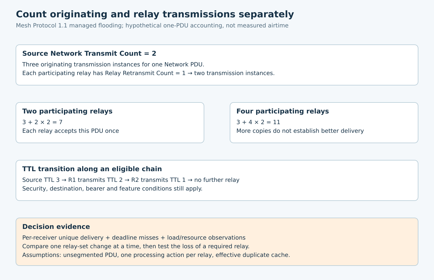
A hypothetical source sends TTL three. Along an eligible chain, relay R1 transmits TTL two and R2 transmits TTL one. A further relay does not extend that copy. This illustrates the field transition, not proof that three particular radio links are reliable.

Too small a TTL can exclude a required route. Raising it permits wider propagation but does not repair missing security configuration, wrong subscriptions or an unreachable gap. Determine a justified operational value through topology and failure tests rather than using the largest value everywhere.

Use approved diagnostics such as heartbeat observations when useful, but keep their traffic and destinations distinct from the application workload. A heartbeat result does not certify delivery of every model message under burst load.

3. Count repetition before counting relays

For a simplified single, unsegmented Network PDU, let the source’s count be two and each participating relay’s count be one. The source schedules three transmissions; each relay schedules two for that relaying action.

If four distinct relays each accept and relay the PDU once, the accounting example is 3 + 4 × 2 = 11 Network-PDU transmission instances. With two participating relays, it is 3 + 2 × 2 = 7. These values compare configured repetition under stated assumptions.

They are not captured advertising-packet counts, airtime totals, delivery probabilities or universal worst-case bounds. Bearer behavior, packet reception, scheduling, multiple channels and other protocol traffic require their own evidence.

The Network Message Cache suppresses repeated processing of recently seen PDUs. Section 3.4.6.5 excludes TTL and NetMIC from duplicate identification because relaying changes them. The cache is finite, with oldest-entry replacement when full; never assume unlimited duplicate memory under arbitrary load.

Therefore, the arithmetic assumes each listed relay processes the PDU only once during the comparison. Record cache sizing and observed repeated-processing behavior separately. Segmentation and application retries multiply different units and are excluded from this first experiment.

4. Compare relay sets without changing everything

Use a controlled installation map with source, required receivers and candidate relay positions. Record enclosure, antenna orientation, power supply, software build, subnet configuration and background traffic. Synthetic application identifiers keep test traffic distinguishable without exposing real users.

1. Verify model binding, destination subscriptions and a low-load baseline before varying relay density.
2. Choose a small relay set that plausibly spans the required area. Fix source repetition, relay repetition, TTL, payload and offered message rate.
3. Run the same workload with one additional relay. Repeat in alternating order so changing interference is less likely to masquerade as improvement.
4. Compare per-receiver unique delivery, deadline misses and observed network load. Keep failed runs in the record.
5. Remove one required relay in an authorized fault test. Determine whether redundancy actually preserves the specified service.
6. Only after comparing relay sets, vary one repetition parameter or interval at a time.

Interval-step fields represent a base interval in ten-millisecond units through (steps + 1) × 10. They are not exact transmit timestamps: the specification describes perturbation and bearer-imposed restrictions. Record actual scheduling evidence before making latency claims.

5. Choose metrics that expose congestion

Attach a generated test-operation identifier and a known destination set. For group delivery, calculate eligible operation–receiver pairs, then count unique completed pairs. Counting all received copies rewards duplication and hides a receiver that never succeeds.

Measure deadline misses and latency distributions alongside eventual delivery. State the clock synchronization or offset bounds before reporting end-to-end latency. Otherwise retain separate source and receiver timing observations.

Track offered load, relay queue pressure or drops where exposed, observed repeated PDUs and application retry attempts. Acknowledged application exchanges add response traffic, so keep acknowledgment behavior fixed while comparing relay sets.

Judge the worst required receiver and failure topology, not only the fleet average. Predefine acceptable delivery, deadline and resource bounds from product requirements. No universal relay count per room or square meter can substitute for those conditions.

6. Save a configuration with a rollback path

The deliverable is a versioned relay-set decision: enabled nodes, read-back counts, TTL scope, workload, tested environments and unresolved gaps. If an added relay improves one edge receiver but pushes burst deadlines beyond the budget, preserve that tradeoff rather than declaring more coverage automatically better.

Roll back through the authorized configuration mechanism and confirm the old state. A useful engineering result explains which relay earns its place, how repetition is bounded and which failures the chosen redundancy actually covers.