Source-Terminated Gateway Clocks: Why the Driver-Side Half Step Is Not a Logic Fault
A gateway board can show an alarming two-step clock waveform beside its driver and a clean transition at the receiving chip. Replacing the series resistor with a short may make the first trace look more familiar while increasing overshoot at the actual receiver. The engineering question is not whether every point on the trace immediately reaches the supply rail. It is whether the intended receiver gets one valid transition within its electrical and timing limits.
This discussion concerns a point-to-point, single-ended clock with a source-series termination and a high-impedance receiving input. It does not prescribe termination for Ethernet pairs, RS-485 cables, or arbitrary clock trees. Texas Instruments’ High-Speed Layout Guidelines, SCAA082A, August 2017 revision, explains propagation delay and reflection coefficients in sections 1.3.1–1.3.2, pages 6–7. Those concepts let us construct a useful numerical model before reaching for a resistor assortment.
Follow the first wave, not the final DC circuit
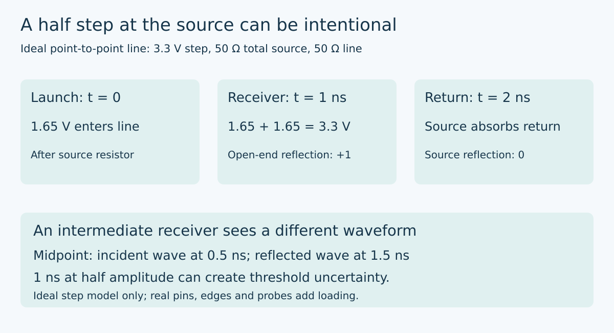
Assume an ideal 3.3 V step source with 15 Ω output resistance, a 35 Ω series resistor immediately beside the driver, and a uniform 50 Ω transmission line. Let the one-way propagation delay be 1 ns. Treat the receiving input as open circuit during the initial wave interaction. These deliberately simple values describe a calculation, not measured gateway hardware or a recommended component combination.
At the instant of launch, the driver sees the line’s characteristic impedance rather than the remote open circuit. The launched voltage is 3.3 × 50 / (15 + 35 + 50), or 1.65 V. That is the voltage immediately after the series resistor. It is not necessarily the voltage measured directly at the driver pin before that resistor; those are different nodes.
At 1 ns, the wave reaches the open end. The load reflection coefficient is +1, so the incident 1.65 V and reflected 1.65 V sum to 3.3 V at the receiver. The reflection then returns toward the source. At 2 ns it reaches the matched 50 Ω source impedance, whose reflection coefficient is zero. No new reflected wave is launched in this ideal model. The line-side source node finally reaches 3.3 V too.
The initial half step is therefore compatible with a full-amplitude first arrival at the intended endpoint. Its existence alone is not evidence of insufficient logic drive. Real edges, receiver capacitance, package inductance, and nonuniform routing smooth or distort this ideal sequence, so use it as a prediction to test rather than a template every capture must exactly match.
Probe location changes the diagnosis
Name three measurement locations on the schematic: the driver pin, the trace immediately after the resistor, and the receiver pin. A screenshot labeled only “clock” cannot distinguish them. Record the probe’s loading and reference connection as well. A long ground connection can introduce a measurement artifact, while probe capacitance can alter the load you are trying to observe.
For the numerical example, a line-side source measurement should show the plateau lasting approximately one round trip. A far-end measurement should first move near the one-way delay and approach the full step on that first arrival. A waveform with a plateau at an intermediate tap is not interchangeable with either endpoint capture. These location-specific predictions make a useful debugging experiment: compare them with identical acquisition settings and a common timing reference, accounting for channel and probe skew.
Do not casually connect an earth-referenced probe to an uncertain industrial potential. The example is a local board-level model; installations with isolation barriers or hazardous voltages require appropriately rated instruments and an approved measurement method.
A resistor cannot rescue an arbitrary fanout
Now imagine adding a second receiving device halfway down the same line. That tap initially sees the incident half-amplitude wave. It does not immediately receive the doubling that happens at the open far end. Its voltage rises again only when the reflected wave returns past it. If its switching threshold lies near the plateau, noise and threshold variation can make the apparent edge timing uncertain.
For a midpoint at half the total delay, the first wave arrives at 0.5 ns. The far-end reflection returns to that midpoint at 1.5 ns. The ideal plateau there lasts 1 ns. This calculation explains why a topology that works for an endpoint receiver may be unsuitable for an additional intermediate clock input, even when both inputs have high DC impedance.
A branch changes the problem further because the wave encounters multiple paths, not a single uniform line. Do not apply the endpoint calculation unchanged to a star connection. Consider a dedicated buffer output and individually designed route for each receiver, or analyze the complete permitted topology with the actual component models. The correct architecture depends on timing, loading, and receiver requirements, not just the number of spare resistor footprints.
Select the resistor from a model with limits
The nominal starting relationship is series resistance plus driver output resistance approximately equal to trace impedance. Driver output resistance is not a universal fixed value: rising and falling behavior and operating conditions can differ. The 35 Ω result above follows only from the assumed 15 Ω source and 50 Ω line.
Obtain the selected driver’s available models and the board fabricator’s stackup information. Include receiver input capacitance, packages, vias, and connectors when their effects matter. Evaluate both transitions at the receiving pin against its input thresholds, allowed overshoot, and clock pulse-width requirements. A slower-looking edge is not automatically better if it violates the receiver’s transition-rate requirements or creates excess timing uncertainty.
The release decision should preserve the reasoning: source impedance assumptions, route topology, expected propagation delay, selected resistor, and receiver-side evidence. Keep source-side captures too, but annotate why their plateau is expected. This produces a reusable design rule for the gateway board instead of an attractive waveform at the wrong node.
Primary reference
- Texas Instruments, High-Speed Layout Guidelines, SCAA082A, revised August 2017, sections 1.3.1–1.3.2, printed pages 6–7. The numerical launch, midpoint, and reflection examples above are independent idealized calculations based on transmission-line relationships, not TI test results.
The preserved Google Trends RISING row “industrial iot solutions,+110%,” worldwide, all categories, web search, July 19–October 19, 2026 motivates the industrial-gateway parent topic only. It does not establish search growth for source termination or this article title.