Gateway ADC Clock Budgets: Use Analog Input Frequency, Not Sample Rate, to Price Jitter

A faster sampling clock does not by itself explain how much signal-to-noise ratio an industrial acquisition gateway loses to timing uncertainty. A slowly varying input and a rapidly varying input can use the same converter clock yet suffer very different voltage errors from the same sampling-time error. Before buying a lower-jitter oscillator, identify the highest relevant analog input frequency and allocate a noise budget at that input condition.

This guide addresses the small-error sinusoidal model for sampling-time jitter. It is useful for gateway acquisition paths handling high-frequency vibration, ultrasound, or other dynamic signals, but it is not a complete model of every converter architecture. Analog Devices tutorial MT-008, copyright 2009, page 2, Figure 2 and Equation 1, gives the jitter-limited SNR relationship. Pages 1 and 3–4 discuss combined aperture/clock jitter and phase-noise integration. The worked numbers below are independent calculations, not measured product performance.

Begin with the slope of the signal being sampled

Write the analog input as A sin(2πft). A small sampling-time error changes the sampled voltage approximately by the local voltage slope multiplied by the timing error. The slope grows with analog frequency f. Thus the same timing error causes a larger voltage error for a faster-changing input even if the sampling rate is unchanged.

For the ideal sinusoidal model, jitter-only SNR in decibels is −20 log10(2πf tj), where tj is total RMS sampling-time jitter in seconds. This is a noise contribution limit, not the total SNR of a real converter. The relationship assumes the relevant random timing-error model and a sufficiently small perturbation. Periodic timing modulation can produce discrete spurs rather than an equivalent flat noise floor.

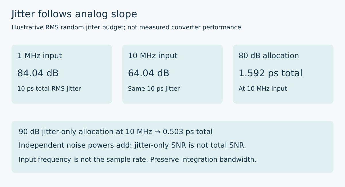
Consider a hypothetical 10 ps total RMS jitter. At a 1 MHz analog input, the formula gives approximately 84.04 dB. At 10 MHz, it gives approximately 64.04 dB. Increasing the input frequency by a factor of ten costs 20 dB in this model. Merely changing the digital output rate in a spreadsheet does not change either calculation unless it also changes the input condition or actual jitter behavior.

For an undersampling design, use the original analog frequency presented to the sampling operation, not the lower frequency at which the tone appears after aliasing. A displayed 100 kHz spectral component may have originated from a much faster input. The sampling aperture still encountered the original waveform slope.

Turn an allocated SNR into a timing limit

Rearranging the equation gives tj = 10^(−SNR/20)/(2πf). For an 80 dB jitter-only allocation at 10 MHz, total RMS timing jitter must be approximately 1.592 ps or less under this model. A 90 dB allocation at the same input requires approximately 0.503 ps.

That ten-decibel improvement is not obtained by subtracting ten percent from the jitter. The logarithmic relationship demands about a 3.162-fold reduction. This is why a loosely stated “high-resolution ADC clock” requirement can create a surprisingly expensive design: neither the analog frequency nor the amount of SNR assigned to timing noise has been fixed.

The useful requirement contains both values. For example, specify the jitter-noise allocation at the highest supported input frequency and the relevant integration conditions, then separately state the total channel SNR objective. Avoid promising the total channel performance from this single limit.

Do not spend the converter’s aperture budget twice

MT-008 describes total jitter as the root-sum-square of internal converter aperture jitter and external clock jitter. That combination applies to independent contributions expressed consistently. Correlated timing errors and periodic components require more careful treatment; simply adding every datasheet number by RSS is not a universal rule.

Suppose a hypothetical converter contributes 1.0 ps RMS aperture jitter, and the allowed total is the 1.592 ps obtained above. The external allowance is the square root of (1.592² − 1.0²), approximately 1.238 ps RMS using unrounded values for the calculation. Assigning the entire 1.592 ps to the oscillator would exceed the intended total once the converter contribution is included.

The external path includes more than the oscillator. A buffer, clock distribution network, power-supply modulation, and threshold-crossing behavior can affect the timing seen by the converter. Use component specifications with compatible conditions, then verify the assembled path. If the converter’s intrinsic contribution already exceeds the total allowance, the square-root argument becomes negative. That is an infeasible allocation, not a reason to report zero required external jitter.

Combine noise powers, not SNR labels

An 80 dB baseline SNR combined with an independent 80 dB jitter-only SNR gives approximately 76.99 dB total, because the two equal noise powers add. The same 80 dB baseline combined with a 90 dB jitter contribution gives approximately 79.59 dB. Both calculations assume the same signal reference and independent noise mechanisms.

This makes “keep jitter above the desired SNR” an incomplete instruction. Decide how much degradation the product can afford, then calculate the required jitter contribution relative to the baseline. A nominal converter resolution is not that baseline. Use the relevant dynamic-performance specification or a properly characterized channel under the intended input and sampling conditions.

Preserve bandwidth when comparing clock specifications

A phase-noise value at one offset is not an integrated time-jitter specification. MT-008 explains integration of phase-noise power across an offset-frequency range and conversion using the clock carrier frequency. That carrier frequency is distinct from the analog input frequency used in the SNR equation.

When comparing clock candidates, keep the integration limits, output frequency, supply, load, and measurement method visible. Two attractive femtosecond figures measured over different offset ranges may not answer the same system question. Check the converter clock-input bandwidth and the application’s sensitivity to close-in effects rather than adopting an integration range merely because it appears in a vendor headline.

The purchasing decision should follow the completed budget: analog operating band, total SNR target, allowable timing-noise contribution, intrinsic aperture term, and external-clock conditions. A lower-jitter part is worthwhile when it resolves a demonstrated allocation, not when it decorates an otherwise unspecified clock tree.

Primary reference and trend scope

Analog Devices, MT-008: Converting Oscillator Phase Noise to Time Jitter, copyright 2009, pages 1–4, especially Figure 2 and Equation 1 on page 2. All example frequencies, jitter allocations, and combined-noise results are hypothetical calculations.

The preserved Google Trends RISING row “industrial iot solutions,+110%,” worldwide, all categories, web search, July 19–October 19, 2026 supports this industrial-gateway parent topic only. It does not establish title-specific demand or growth in ADC-clock searches.