Gateway Buck Regulators: Check Frequency Foldback at High Input Ratios
A buck regulator can maintain its output voltage while no longer switching at the frequency printed in the design summary. At a high input-to-output ratio, the requested high-side pulse may become shorter than the controller can produce. Some regulators respond by reducing switching frequency. That can be valid operation, but it changes the assumptions used for ripple, filtering and interference analysis.
Texas Instruments LMR33630 datasheet SNVSAN3F, revised November 2020, documents this behavior in section 8.4.3. The calculations below use an explicitly hypothetical 80 ns minimum on-time to show the boundary. That value is not a guaranteed LMR33630 timing specification, and the arithmetic is not a tested converter design.
Translate the conversion ratio into time
For an ideal continuous-conduction buck, duty ratio is approximately VOUT/VIN. On-time is duty ratio divided by switching frequency. This converts a voltage-ratio question into a timing requirement that can be compared with the selected regulator’s limits.
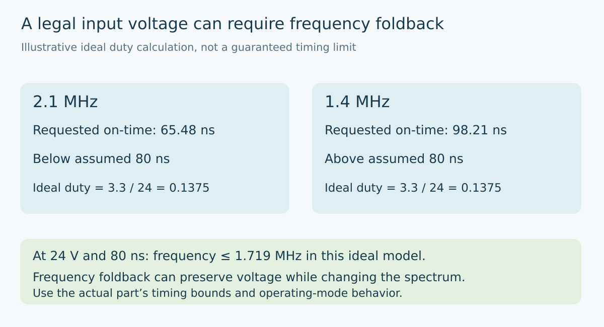
Consider a hypothetical 24 V input and 3.3 V output. Ideal duty ratio is 0.1375. At 2.1 MHz, the switching period is approximately 476.19 ns and the requested on-time is 65.48 ns. At 1.4 MHz, the same voltage ratio requires approximately 98.21 ns.
If a hypothetical controller could not generate a pulse shorter than 80 ns, the first operating point would require behavior beyond ordinary fixed-frequency PWM. The second point would satisfy that particular ideal timing comparison. Neither result establishes complete regulation, because losses, operating mode and actual controller limits remain outside the simple equation.
This distinction helps separate two statements often merged in a schematic review: the input voltage is inside the device’s allowed range, and the converter will retain its nominal switching frequency there. The first does not automatically establish the second.
Calculate the frequency boundary
Rearranging the ideal relationship gives f ≤ VOUT/(VIN × tMIN) for operation without demanding a shorter on-time. With 3.3 V, 24 V and the hypothetical 80 ns constraint, the boundary is approximately 1.719 MHz.
At a 32 V input with the same output, the boundary falls to approximately 1.289 MHz. At 2.1 MHz, the requested on-time would be only 49.11 ns. A design checked solely at nominal 24 V could therefore understate the timing pressure at the upper end of its operating range.
An equivalent calculation solves for input voltage: VIN ≤ VOUT/(tMIN × f). At 2.1 MHz and the same assumptions, that gives approximately 19.64 V. This is the boundary of this ideal fixed-frequency model, not a maximum permitted input voltage or an absolute device rating.
Keep the assumed timing value prominent in the calculation sheet. A typical number describes neither a guaranteed worst-case bound nor every temperature and operating condition. Use the selected device’s actual specification and documented estimation method when converting this screening example into a product decision.
Interpret foldback as a mode change
The LMR33630 documentation explains that switching frequency decreases when the minimum on-time limit is reached, allowing regulation at low output voltage and high input voltage. Its Figure 8-13 illustrates that transition. The architectural lesson is that a stable output does not prove fixed-frequency operation.
Do not generalize that behavior to all bucks. Another controller may use a different pulse-management strategy, impose a different conversion boundary or have a different permitted operating envelope. The appropriate diagnosis comes from the exact part and mode, not from the generic label “switching regulator.”
Likewise, distinguish high-ratio foldback from light-load behavior. A waveform containing fewer switching events may have several explanations. Record input voltage, output load, operating-mode configuration and the on-time of the remaining pulses before assigning the cause.
A useful proposed comparison holds load constant while sweeping input within the permitted low-voltage range. A second comparison holds input constant while changing load. These independent axes help distinguish a conversion-ratio boundary from a load-dependent transition. They are planned observations, not reported measurements.
Revisit ripple at the actual frequency
The ideal buck ripple expression is ΔI = (VIN − VOUT) × VOUT/(VIN × L × f). Under otherwise unchanged assumptions, reducing frequency increases ripple. Therefore, an inductor calculation made at nominal frequency can become optimistic if the converter spends part of its required range below that frequency.
For a hypothetical 24 V to 3.3 V conversion with 10 µH, the expression gives approximately 0.1355 A peak-to-peak at 2.1 MHz. At 1.4 MHz it gives approximately 0.2033 A peak-to-peak. These are ideal continuous-conduction comparisons, not predictions for a particular foldback waveform or recommended inductance.
If operation becomes discontinuous, or the pulse sequence departs from the assumed periodic waveform, use the appropriate model instead. Do not feed an average event rate into a fixed-period ripple formula and silently claim an exact result. Preserve the actual timing sequence when evaluating voltage ripple or spectral behavior.
Qualify the spectrum you actually generate
Filtering and interference plans should cover the observed or justified frequency range, not only the nominal oscillator setting. A sensitive measurement path may encounter a switching component at a different frequency under high input voltage even though the output remains within its DC tolerance.
That possibility is not a claim that emissions necessarily worsen. It means the qualification conditions need to include the mode transition. Check the intended supply range, load range and relevant thermal conditions, retaining both rail behavior and switching timing. Use suitable current-limited low-voltage equipment and measurement methods appropriate to the board.
Record whether fixed frequency is a functional requirement or merely an initial design assumption. If the application requires a bounded switching band, select an architecture and operating envelope that support it. If foldback is acceptable, incorporate its consequences into the inductor, output-capacitor and filter review instead of labeling every departure from nominal frequency a fault.
The final acceptance statement should distinguish voltage regulation from switching-mode consistency. Both may be satisfactory, but they need separate evidence. A DC voltmeter can establish neither the requested pulse width nor the spectrum produced when that pulse becomes too short.
Primary reference and trend scope
The preserved Google Trends RISING row “industrial iot solutions,+110%,” worldwide, all categories, web search, July 19–October 19, 2026 supports the parent integration topic only. It does not establish search growth for minimum on-time or this article title.