Aligning Logic Analyzer and Firmware Logs: State the Timestamp Uncertainty Before Measuring Latency

Align firmware and logic-analyzer records through identifiable common events, then state the uncertainty of that alignment before subtracting timestamps. One marker can establish an offset under a clock-rate assumption. Two separated markers can estimate a rate difference, but they do not prove that the mapping remained valid between them or across a reset.

This article uses Saleae’s official timing-error and clock-comparison guidance as inspected on 14 October 2026. An original exact-rational Python 3.12.14 calculation checks a hypothetical two-anchor map and latency interval. No analyzer, GPIO or firmware timing measurement was performed, and the example uncertainty bounds are chosen assumptions.

Name both clock domains and both events

Record the firmware counter’s units, frequency source, width, wrap behavior, reset epoch and any frequency changes. Record the analyzer model, capture rate, channel configuration and timebase specification. Two columns expressed in microseconds are not necessarily on the same scale or origin.

Define the latency endpoints physically. For example, one endpoint could be a firmware event associated with a diagnostic GPIO edge, while the other is an externally observed response. A timestamp taken when a log line reaches the host measures a different event and includes transport and buffering delay.

Document where the firmware reads its clock relative to writing the marker. The marker instruction, peripheral path and electrical transition can add delay and variation. Do not assume that two neighboring source-code statements occur at the same instant.

Create recognizable common anchors

Use an electrically approved diagnostic signal or another event visible in both records. Give each anchor an identity so missing pulses cannot shift the alignment by one event. A distinctive pattern can help recognition, but the pattern must still be associated with the correct firmware record.

Place anchors around the interval of interest rather than only at startup. Capture them under the same clock mode and representative workload. Avoid choosing an anchor whose instrumentation cost overwhelms the latency being investigated.

Saleae’s clock-comparison guidance calls attention to channel-to-channel skew and matching transition records. Those concerns remain relevant when an analyzer channel is compared with firmware logs: the correspondence and measurement path must be established before a numerical difference has meaning.

Fit a bounded two-anchor mapping

Let F be firmware ticks and A be analyzer seconds. For paired anchors (F0, A0) and (F1, A1), use the illustrative affine map A(F) = A0 + (F − F0) × (A1 − A0) / (F1 − F0). Reject equal firmware anchors and do not combine points from different counter epochs.

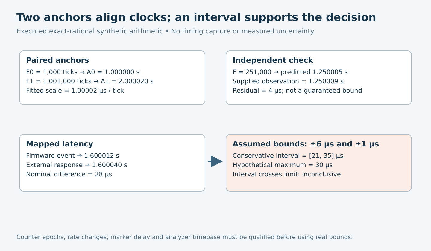
In the synthetic calculation, F0 is 1,000 ticks at A0 = 1.000000 seconds. F1 is 1,001,000 ticks at A1 = 2.000020 seconds. The resulting scale is 1.00002 microseconds per tick. At F = 501,000, the mapped time is 1.500010 seconds.

This fitted scale describes the relationship between the two supplied clocks. It does not identify which oscillator is more accurate, certify either clock against an external standard or establish a constant rate outside the anchor interval.

Check an independent marker rather than admiring the fit

A line through two anchors necessarily matches both anchors. Keep at least one other recognizable event outside the fit and compare its observed analyzer time with the predicted time. Inspect residuals over the interval and after changes in temperature, clock configuration or power state.

The model’s independent marker at F = 251,000 maps to 1.250005 seconds. Its deliberately supplied analyzer observation is 1.250009 seconds, leaving a 4 microsecond residual. That number is synthetic. It illustrates a check that the endpoint fit alone would hide.

One residual does not establish a guaranteed uncertainty envelope. It can reveal a problem, but the bound still needs evidence for anchor placement, counter quantization, drift, marker delay and instrument behavior. A maximum observed residual from a finite campaign is not automatically a worst-case bound.

Build the uncertainty ledger

Contribution	Evidence needed
Analyzer sampling and timebase.	Actual model/specification, sample rate, capture duration and operating conditions.
Channel and probe path.	Applicable skew, threshold, loading and transition behavior.
Firmware clock capture.	Counter quantization, read location, epoch and frequency stability.
Marker relationship.	Bounded delay between the intended event, clock read and observable edge.
Mapping residual and extrapolation.	Independent markers and justified limits over the reported interval.

Saleae’s timing-error explanation separates sample-clock error from asynchronous-sampling uncertainty. Its idealized two-edge interval discussion gives a one-sample-period uncertainty in either direction under stated assumptions about digital transitions and clock jitter. Do not reuse that one term as the complete uncertainty of a firmware-to-analyzer measurement.

Keep deterministic bounds and statistical estimates labeled. Adding compatible absolute bounds conservatively is different from combining standard uncertainties under a justified statistical model. Do not select a root-sum-square calculation merely because it produces a smaller number.

Turn the mapped latency into a decision interval

The synthetic firmware event at F = 601,000 maps to 1.600012 seconds. An external response at 1.600040 seconds gives a nominal latency of 28 microseconds. Exact rational arithmetic verified these values without floating-point rounding ambiguity.

Now assume, purely for illustration, that the mapped event has a qualified ±6 microsecond bound and the external event has ±1 microsecond. Their conservative combined bound is ±7 microseconds, producing a latency interval from 21 to 35 microseconds.

Against a hypothetical 30 microsecond maximum requirement, that interval crosses the boundary. The example cannot establish a pass even though the nominal value is below 30. The six-microsecond mapping bound was not derived from the four-microsecond residual; both are separately supplied illustrative inputs.

Invalidate the map when its assumptions change

Start a new mapping after firmware reset, ambiguous counter wrap, clock-source or rate changes, or a capture discontinuity. Do not stretch one affine model across a sleep interval whose counter behavior is unknown. If extrapolation is necessary, state the additional uncertainty and its basis.

Deliver paired raw anchors, independent residuals, clock definitions, instrument settings, event meanings and the final decision interval. If the uncertainty is too large for the requirement, improve the observation path or use a qualified shared-clock/hardware-capture design. Extra decimal places cannot supply missing timing evidence.