Aliasing in Periodic Sensor Acquisition: Do Not Mistake a Slow Trace for a Slow Signal
A slow-looking sensor trace can be an alias of a much faster input. Establish the actual conversion cadence, identify unwanted frequencies that can reach the sampler, and test the apparent component while changing a controlled acquisition parameter. A smooth chart and a larger moving average cannot establish that the original physical signal was slow.
Applicability: This procedure addresses periodic, baseband acquisition with an approximately uniform sample clock. The theory reference is Analog Devices MT-002, Revision A, October 2008; Linux buffer behavior is referenced to v6.12. Intentional bandpass sampling, irregular sampling reconstruction, and a particular sensor’s internal digital filters require separate models. The frequency examples are mathematical hypotheticals, not measurements.
1. Identify where sampling actually occurs
Draw the path from physical stimulus through sensor dynamics, analog conditioning, conversion, internal filtering, output registers, host reads, and presentation. Write a rate beside every boundary that creates or discards samples. A host reading a continuously converting sensor periodically does not necessarily control the converter’s sample clock.
Distinguish conversion rate, per-channel rate in a multiplexed scan, device output rate, buffer delivery rate, and display refresh rate. A multichannel aggregate throughput cannot automatically serve as each channel’s sampling frequency. Identify whether reading the register repeats the last result or starts another conversion.
For example, the Linux v6.12 IIO buffer interface separates buffered samples from read and poll behavior, including watermark handling. A burst delivered to userspace is not evidence that the physical samples were acquired simultaneously. Obtain timing evidence at the conversion or documented trigger boundary.
2. Predict a plausible alias before experimenting
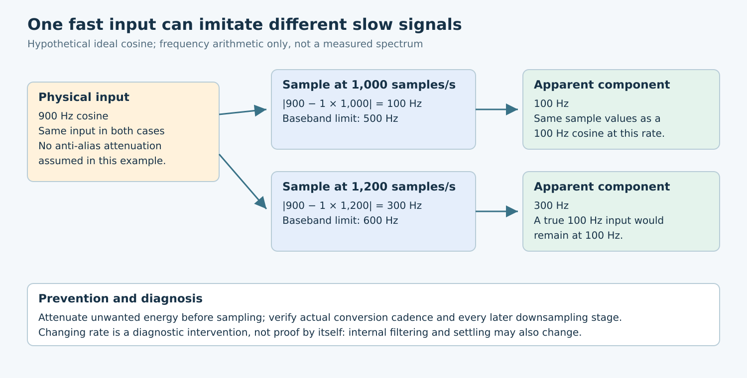
For a single tone at frequency f and uniform sampling at fs, find an integer k for which |f − kfs| lies between zero and fs/2. That gives its baseband alias frequency. MT-002’s Nyquist-zone discussion explains the repeated spectral images and why components outside the intended band can fold into it.
Consider a hypothetical 900 Hz cosine sampled at 1,000 samples per second. Its samples equal those of a 100 Hz cosine with zero initial phase: cos(2π × 900n/1000) equals cos(2π × 100n/1000) for integer n. These two inputs cannot be distinguished from those sample values alone.
At 1,200 samples per second, the same 900 Hz tone folds to 300 Hz. A genuine 100 Hz tone remains at 100 Hz under ideal sampling. This arithmetic suggests a useful experiment; it does not prove that an observed component came from a specific interference source.
3. Assemble a controlled stimulus-and-rate matrix
- Capture the original condition: save raw samples, actual timing information, configuration, and the processing chain that produced the suspicious trace.
- Apply an in-band reference: use a suitable independent stimulus within the complete signal path’s operating limits. Check that the expected frequency survives without clipping or unexplained rescaling.
- Apply a suspected out-of-band component: predict its aliases at several permitted conversion rates before taking data.
- Change one actual sample rate: confirm that the hardware accepted it. Keep input conditions and other processing fixed where possible.
- Repeat with changed analog attenuation: use an approved filter configuration and compare the suspicious component with its predicted attenuation.
Choose record duration and analysis settings that resolve the frequencies being compared. Record windowing, detrending, and amplitude conventions if using an FFT. Leakage from a finite record can spread a tone across bins; it is a different mechanism from aliasing. A fitted time-domain frequency can be useful too, but its assumptions must be stated.
Changing a device rate can also change its internal filter, noise, power state, or signal settling. If several properties move together, the experiment is confounded. Record those changes and avoid attributing every moving spectral peak to aliasing.
4. Place attenuation before the vulnerable sampling boundary
For ordinary baseband acquisition, constrain the spectrum reaching the sampler and leave a realizable transition region between the wanted band and frequencies requiring rejection. MT-002 discusses this filter/sample-rate tradeoff. “Sample above twice the wanted frequency” is incomplete when substantial unwanted energy remains outside that wanted band.
Build a small interference table: source or frequency range, largest credible input amplitude, predicted fold location, allowable in-band error, and required attenuation. Derive the attenuation from that budget. Do not select a universal cutoff, resistor, or capacitor without the chosen sensor, ADC input model, source impedance, and component tolerances.
A network used to settle a switched-capacitor input may not provide sufficient rejection at relevant alias frequencies. Check its transfer function and acquisition interaction separately. A nominal bandwidth label is weaker evidence than the response over the entire interference range under actual loading.
Digital filtering can protect a later rate-reduction stage when applied before that decimation. It cannot generally separate an unwanted component already folded onto a wanted component by an earlier sampler. Identify every downsampling boundary rather than assigning all responsibility to one final software filter.
5. Interpret results without overstating them
| Observation | Next interpretation check |
|---|---|
| Component moves as the predicted alias moves | Check independently that the source frequency and actual sample rate stayed as intended. |
| Component shrinks with added analog rejection | Check that wanted-band gain and input settling did not change enough to explain it. |
| Only the plotted trace changes | Compare raw data and presentation processing before changing hardware. |
| Timing is irregular or samples are missing | Repair the timing model before interpreting a uniform-sampling spectrum. |
Also test interference from clocks, switching supplies, and mechanical sources that vary with operating state. A quiet laboratory input does not bound every installation. Keep the generator and reference instrument limitations in the evidence record, especially their bandwidth, loading, and frequency accuracy.
6. Deliver an acquisition argument
The useful output is a rate map, a predicted-alias table, a filter attenuation budget, and captures that test the proposed mechanism. Separate specified component behavior, calculated frequencies, and board observations. Preserve enough configuration to reproduce the acquisition, not just an exported chart.
No hardware acquisition or spectral test was performed for this article. Acceptance means that plausible out-of-band energy is sufficiently rejected at each vulnerable sampling boundary and that the remaining interpretation agrees with independent stimulus and timing evidence. A believable slow waveform alone is insufficient.