Measuring Sleep Current Across Large Bursts: Do Not Let Instrument Range Changes Hide Energy

Choose a current instrument by the smallest idle signal, largest burst, transition speed, and permitted disturbance to the supply. Then verify that the recorded data preserves charge across range changes. A readable low-current display does not prove that short bursts are captured, and a flattened peak does not automatically mean its energy was lost.

Applicability: Nordic Power Profiler Kit II (PPK2) is the concrete instrument, using the official online user guide whose latest listed revision is May 2025, inspected on 14 October 2026. The arithmetic fixture below is hypothetical and is not a PPK2 error measurement. Firmware, application version, calibration state, and actual wiring must be recorded for any real test.

1. Translate the workload into measurement requirements

List the expected idle range, peak current, shortest important pulse, repetition interval, supply voltage, and energy window. Include startup and recovery bursts, not just normal sensing. Decide whether the question is peak amplitude, pulse duration, charge, or energy; one instrument configuration may not answer all four with the same uncertainty.

The PPK2 guide specifies 100 kS/s sampling and five automatically selected current ranges. The nominal sample interval is therefore 10 microseconds. This calculation is not an analog-bandwidth specification or a promise to reconstruct every pulse shorter than that interval.

For a proposed test, a 100-microsecond pulse spans roughly ten nominal sample periods. Its alignment to the sample grid, analog response, and data processing still matter. Vary the pulse phase or repetition timing rather than using only a perfectly synchronized waveform that can conceal phase sensitivity.

2. Keep resolution, accuracy and switching behavior separate

The PPK2 resolution table lists a typical 0.2-microamp resolution in its 200 nA–50 µA range, while the 50–1000 mA range lists 1000 µA. A headline resolution from the lowest range is not the resolution available during a large burst.

The separate accuracy table describes typical average-value readout accuracy. Those entries do not establish a worst-case accuracy for every individual transient sample. Record each applicable specification with its conditions rather than combining the most attractive number from each table.

The measurement-system description confirms automatic selection among five measurement ranges. It does not provide, in that description, a universal zero-error transition guarantee. Conversely, automatic ranging is not evidence that samples are necessarily missing. Treat transition behavior as a qualification question, not a presumed defect.

3. Check whether the instrument changes the workload

Choose Source Meter or Ampere Meter mode deliberately. The PPK2 power-supply instructions state that Ampere Meter mode uses an external supply applied without regulation and limits that voltage to 0.8–5.0 V. The instrument’s current range is not permission to exceed its voltage limits.

Measure the voltage at the DUT during bursts using a suitable independent method. Include lead resistance, connectors, measurement insertion, and supply response in the setup review. A current trace with missing bursts may reflect a target that resets or never transmits under the altered supply, rather than lost samples in the recorder.

Define where current is measured relative to local capacitors. A capacitor downstream of the instrument can supply a fast load edge while the upstream measurement sees recharge spread over time. For charge accounting, include the recharge interval and comparable initial and final capacitor states. For peak-load analysis, the upstream trace alone may answer a different question.

4. Use a charge fixture that makes lost intervals visible

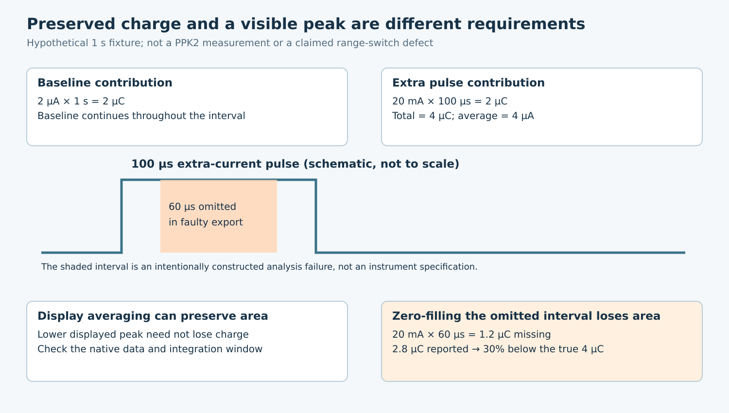
Consider a hypothetical one-second workload with a constant 2 µA baseline plus an additional 20 mA pulse lasting 100 µs. Baseline charge is 2 µC; the extra pulse also contributes 2 µC. Total charge is 4 µC, so the time-average current is 4 µA.

A plot that averages the pulse into a wider display bucket can show a much lower maximum while preserving the same integrated charge. By contrast, if a deliberately constructed faulty export omits 60 µs of the extra pulse and treats it as zero, it loses 1.2 µC. The reported total becomes 2.8 µC, a 30% underestimate. This is an arithmetic counterexample, not an observed PPK2 behavior.

Use such a fixture to review the analysis pipeline. Invalid or missing samples must remain marked; do not silently replace them with zero or bridge them with an attractive line. If bounding the omitted charge requires an unknown peak, report the result as incomplete rather than assigning an unjustified precise total.

5. Qualify transitions and the exported data together

Propose a controlled load that can produce steady levels and repeatable pulses within the instrument’s ratings. Independently characterize its current and timing. Sweep levels around relevant range regions and include upward and downward transitions, long dwell times, short bursts, and the product’s real quiet-to-active pattern.

Compare the native captured data with any exported or downsampled representation. Check timestamps, duration, sample continuity, units, validity flags, and the integration convention. A screen capture is useful for orientation but cannot replace retained numerical data when charge is the acceptance quantity.

Use a separate reference appropriate to the question. A slow average-current measurement can cross-check a repeated pattern’s mean while remaining unsuitable for its peak. A higher-bandwidth capture may expose edge shape while introducing its own burden and offset. Record those limits rather than declaring either instrument an unquestioned truth source.

6. Make the acceptance decision explicit

Set separate tolerances for idle-current discrimination, burst charge, total cycle charge, and supply disturbance. Reject a configuration that clips peaks, loses unbounded intervals, or changes the DUT’s functional behavior. A stable average can still conceal the wrong application workload, so retain event markers and success counts alongside the electrical data.

For energy, integrate voltage times current over the same window. Multiplying charge by one voltage is justified only when that voltage is a suitable representation of the actual supply for the required accuracy. Do not turn a nominal battery label into a measured energy trace.

The final report should identify the instrument and software versions, measurement mode, range-dependent limits, raw and exported files, analysis method, and unresolved uncertainty. That evidence supports an instrument-suitability decision. It does not, without real DUT measurements, establish a power saving or battery runtime.