Conductivity Gateway Inputs: Check Excitation Symmetry Before Trusting a Stable Reading

An electrical conductivity channel can report a steady value while its excitation applies an unwanted average voltage to the probe. The ADC may be behaving correctly; the instrument is changing the conditions it is supposed to measure. For an industrial liquid-monitoring gateway, the waveform at the cell is part of the measurement contract, not merely an internal clock setting.

Alternating excitation helps address electrode polarization, but the label “AC” is incomplete. Unequal positive and negative amplitudes, unequal dwell times, or an interrupted waveform can leave a DC component. A nominally symmetric PWM configuration does not establish that the analog output seen by the cell is symmetric.

Why the excitation deserves its own review

Analog Devices’ CN-0359 uses programmable alternating excitation with low residual DC content. Its discussion of electrolysis and polarization explains why the applied level and frequency must suit the selected conductivity cell. It also emphasizes minimizing DC content rather than treating any periodically changing voltage as acceptable excitation.

The reference design’s component choices and reported performance apply to that design. They are not limits for an arbitrary probe or gateway. Obtain the cell manufacturer’s supported excitation conditions and define the desired measurement range before selecting an amplitude, frequency, or waveform.

The practical distinction is between observing a liquid property and disturbing the electrode interface. A resistor substituted for the cell can help verify acquisition gain, but it does not reproduce electrode polarization or the solution’s electrochemical response. Passing a resistor check therefore answers only part of the instrument question.

Calculate the average of the waveform you actually generate

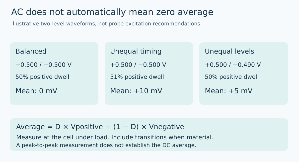
For a two-level waveform, let the positive level be Vp, the negative level be Vn, and the fraction of the cycle spent at Vp be D. Its average is D × Vp + (1 − D) × Vn. Here Vn is a signed negative voltage, not a positive magnitude.

With ideal +0.5 V and −0.5 V levels at a 50% duty cycle, the average is zero. If the positive dwell becomes 51% while the levels remain unchanged, the average becomes +10 mV. If the dwell is exactly 50% but the levels are +0.500 V and −0.490 V, the average is +5 mV.

These are illustrative arithmetic examples, not recommended excitation levels or acceptable residual offsets. They show two independent mechanisms. Correcting timer duty cycle does not correct unequal analog levels, and matching the analog levels does not correct unequal dwell times.

Real waveforms also have transitions, settling, and possible clipping. When those intervals are material, evaluate the time integral over a complete cycle rather than assuming an ideal two-level shape. The waveform relevant to the cell can differ from the unloaded driver output or the MCU pin.

Keep measurement amplitude separate from DC balance

A synchronous measurement may extract a difference between positive and negative observations. That difference can provide useful signal amplitude while discarding their average. In the +0.500 V/−0.490 V example, the peak-to-peak difference is 0.990 V even though the waveform has a +5 mV mean.

A measurement path that accurately captures the difference does not automatically prove that the mean is negligible. Preserve a way to evaluate both quantities during development. Similarly, an AC-coupled oscilloscope view can make the waveform look centered while concealing the DC component being investigated.

Document the instrument input mode, probe loading, bandwidth, and reference connection used to observe the excitation. The goal is a waveform measurement under the intended load, not an attractive screenshot of an unloaded logic signal. Choose equipment and connections suitable for the actual circuit limits.

Sample timing is another independent condition

CN-0359 uses synchronous sampling of the positive and negative portions of the excitation. In a custom implementation, sampling too near an edge can mix settling behavior into the measured current or voltage. A perfectly balanced waveform does not ensure that two samples represent equivalent settled conditions.

Describe sample timing relative to the actual excitation transitions. If the design changes excitation frequency or acquisition gain, check whether the same timing relationship remains valid. Do not assume that preserving the sample count per cycle preserves the available settling interval.

A useful diagnostic captures the voltage and current observation windows on the same time base as the excitation. Distinguish a changing cell response from a window that moved into a transition. This is a targeted timing check, not a claim that every conductivity error is caused by synchronization.

Startup and interruption are part of the waveform

A periodic steady-state calculation does not describe startup, range changes, processor resets, or a paused driver. If one excitation polarity remains applied while firmware stops, the cell no longer sees the intended alternating pattern.

Define the permitted electrical state for these transitions using the probe and front-end requirements. Consider whether the hardware and firmware together reach that state when acquisition is suspended. The appropriate state is architecture-dependent; this article does not prescribe shorting a cell, leaving it connected, or using a universal timeout.

Review both sides of a range change. A new amplitude with an old current-range setting may clip one portion of the cycle before the normal measurement resumes. Mark affected results unavailable rather than treating the first plausible numerical value as proof that the excitation and acquisition have both settled.

Separate the three pieces of evidence

The electronics evidence should establish voltage/current scaling and timing using suitable electrical fixtures. The excitation evidence should establish the actual cell-terminal waveform, including average content and relevant transitions. The probe evidence should establish suitability and calibration with the intended cell and application conditions.

Keep the cell constant and temperature handling traceable in the final conversion, but do not use those numerical corrections to conceal an unexplained excitation asymmetry. A stable displayed conductivity is not a substitute for knowing which physical waveform produced it.

No conductivity tests or chemical qualification are reported here. The design outcome is a bounded excitation contract: supported probe, waveform limits, sampling relationship, and transition behavior. That contract gives a gateway team a more useful starting point than simply declaring that the input uses AC.

Primary reference and trend scope

Analog Devices CN-0359, Revision C, Excitation Generation and Preventing Electrolysis and Polarization provides the circuit context. Average-voltage examples and integration checks above are original analytical recommendations.

The parent topic follows the preserved Google Trends RISING row “industrial iot solutions,+110%,” worldwide, all categories, web search, July 19–October 19, 2026. This does not claim title-specific or conductivity-sensor search growth.