IEPE Vibration Inputs: Choose the Coupling Pole Before Promising Low-Frequency Response

An IEPE vibration sensor presents a dynamic signal riding on a DC bias. Removing that bias makes the signal easier to accommodate in a gateway’s ADC path, but the chosen removal method also shapes what the gateway can observe. An AC-coupled input may look excellent at a convenient calibration frequency while attenuating and phase-shifting the low-frequency content the application actually needs.

The design decision is therefore not simply “capacitor or no capacitor.” It is the relationship between the lowest useful frequency, permitted amplitude and phase error, and the time the channel needs after a disturbance. State those requirements before turning a capacitor value into a product bandwidth claim.

Separate sensor bandwidth from acquisition bandwidth

Analog Devices’ CN-0540 describes a DC-coupled IEPE signal chain that accommodates sensor bias. Its AC-versus-DC discussion explains that inserting a coupling capacitor changes the input to a high-pass response. The document also identifies the additional DC and low-frequency capability as a reason for the DC-coupled architecture.

That does not mean that a DC-coupled gateway turns every piezoelectric accelerometer into a sensor of static acceleration. The sensor’s own frequency response remains part of the chain. Likewise, a sensor with adequate low-frequency response cannot recover content that the gateway’s coupling network has already attenuated.

Write the two responses separately in the interface review. One belongs to the selected sensor and its operating conditions. The other belongs to the acquisition path, including its analog coupling and digital filtering. A system response needs both, not whichever component has the more attractive bandwidth number.

Use an explicit first-order model

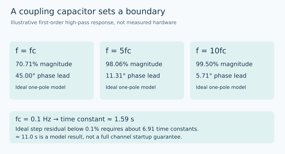
For an ideal first-order AC-coupling high-pass network, let fc be its cutoff frequency and let x equal signal frequency divided by fc. The magnitude relative to the high-frequency gain is x divided by the square root of one plus x squared. Its phase lead is arctangent of one divided by x.

At the cutoff, the magnitude is about 0.7071 and phase lead is 45 degrees. At five times the cutoff, the magnitude is approximately 0.9806 and phase lead is 11.31 degrees. At ten times the cutoff, the magnitude is approximately 0.9950 while the phase lead is still 5.71 degrees.

These are calculated values for a model, not measurements from CN-0540 or an Obeita board. They demonstrate why an amplitude-only check can miss a phase requirement. A response already within roughly half a percent of its high-frequency magnitude can still have several degrees of phase shift.

The relevant resistance for fc = 1/(2πRC) is the effective resistance seen by the capacitor in the implemented network. Do not insert a convenient resistor value from the bill of materials without checking the source, bias network, and following stage. Additional poles and zeros require the actual transfer function rather than this one-pole shortcut.

Work backward from the required measurement

Suppose an application requires no more than 1% amplitude loss from this one coupling pole at its lowest measurement frequency. Solving the magnitude expression for a minimum gain of 0.99 gives a frequency ratio of approximately 7.02. Thus the cutoff must be no higher than the lowest measurement frequency divided by about 7.02, before allowing for tolerances or other response errors.

A separate limit of five degrees of phase shift would require a ratio of at least 1/tan(5°), approximately 11.43. In that illustrative case, the phase allocation is stricter than the amplitude allocation. The requirement, not a customary capacitor size, decides which boundary controls the choice.

These allocations also belong to this stage alone. If the sensor, analog anti-alias filter, or digital processing consumes part of the system error allowance, the coupling stage cannot consume the entire allowance again. Keep the phase reference and any channel-to-channel matching requirement explicit.

A lower pole has a time-domain cost

For the same ideal model, the time constant is 1/(2πfc). A cutoff of 0.1 Hz corresponds to approximately 1.59 seconds. Following an ideal step, the transient component decays exponentially. Reaching a residual below 0.1% of its initial value takes about 6.91 time constants, or approximately 11.0 seconds in this example.

That calculation is not a complete startup guarantee. Real bias establishment, input overload, amplifier recovery, sensor settling, and software filtering can add other behavior. It does show why reducing the coupling pole can conflict with a short “data valid after connection” requirement.

Express validity relative to the intended measurement, not merely to elapsed time. A channel that has recovered enough for a large vibration signal might still have excessive transient content for a small low-frequency measurement. A fixed delay copied from another sensor or gain setting needs evidence before being reused.

DC coupling moves rather than removes the design problem

A DC-coupled path must accommodate or compensate the sensor’s bias while retaining room for the useful waveform. Review the supported bias range, signal excursion, converter range, and recovery behavior in the actual architecture. Subtracting an offset from digitized values cannot recover peaks that were clipped before conversion.

Conversely, do not assume an AC-coupled channel is immediately ready simply because its settled output is centered correctly. Bias changes can produce transients through the coupling network. A useful comparison of the architectures includes low-frequency response and recovery requirements, not only settled noise or nominal resolution.

The interface specification should identify the allowed sensor family, acquisition response, amplitude and phase limits over the required band, and conditions that make samples temporarily unusable. Keep analytical predictions separate from measured results. This article supplies a decision model, not an environmental qualification or a claim of tested product performance.

Primary reference and topic provenance

Analog Devices, CN-0540, Revision A, AC- vs. DC-Coupled Solution provides the IEPE architectural context. The single-pole response, requirement inversion, and settling calculations above are original analytical examples and do not reproduce that reference design’s measured response.

The topic follows the preserved Google Trends RISING row “industrial iot solutions,+110%,” worldwide, all categories, web search, July 19–October 19, 2026. That evidence concerns the parent industrial-integration topic, not rising demand for IEPE sensors or this particular article.