TinyML Weight Compression: Trade Flash Savings Against Arena Memory and Inference Work

A compressed TinyML model is smaller in storage but fails to fit the runtime arena. That can be an expected tradeoff: the examined TFLM lookup-table compression stores compact indices and reconstructs tensor values into writable memory when a kernel needs them.

Evaluate compressed model bytes, decompression workspace and execution cost separately. This article concerns the specific upstream compression facility, not arbitrary ZIP compression of a model file or a promise that every microcontroller backend supports it.

Check the supported path before estimating savings

The pinned compression guide lists support for X86 and specified Xtensa targets. It lists particular kernels, including fully connected and convolution variants. That list does not establish general Cortex-M or CMSIS-NN coverage.

Confirm that the selected kernel implementation understands compression, not merely that its operator name appears in the model. An optimized backend can use a different implementation from the reference kernel. Unsupported compressed constants are an integration boundary, not a reason to reinterpret packed bytes as ordinary weights.

Account for the lookup table as well as packed indices

The compression metadata schema associates a tensor with a value-table buffer and an index bit width. The tensor's logical dimensions remain meaningful even though its stored payload contains packed indices.

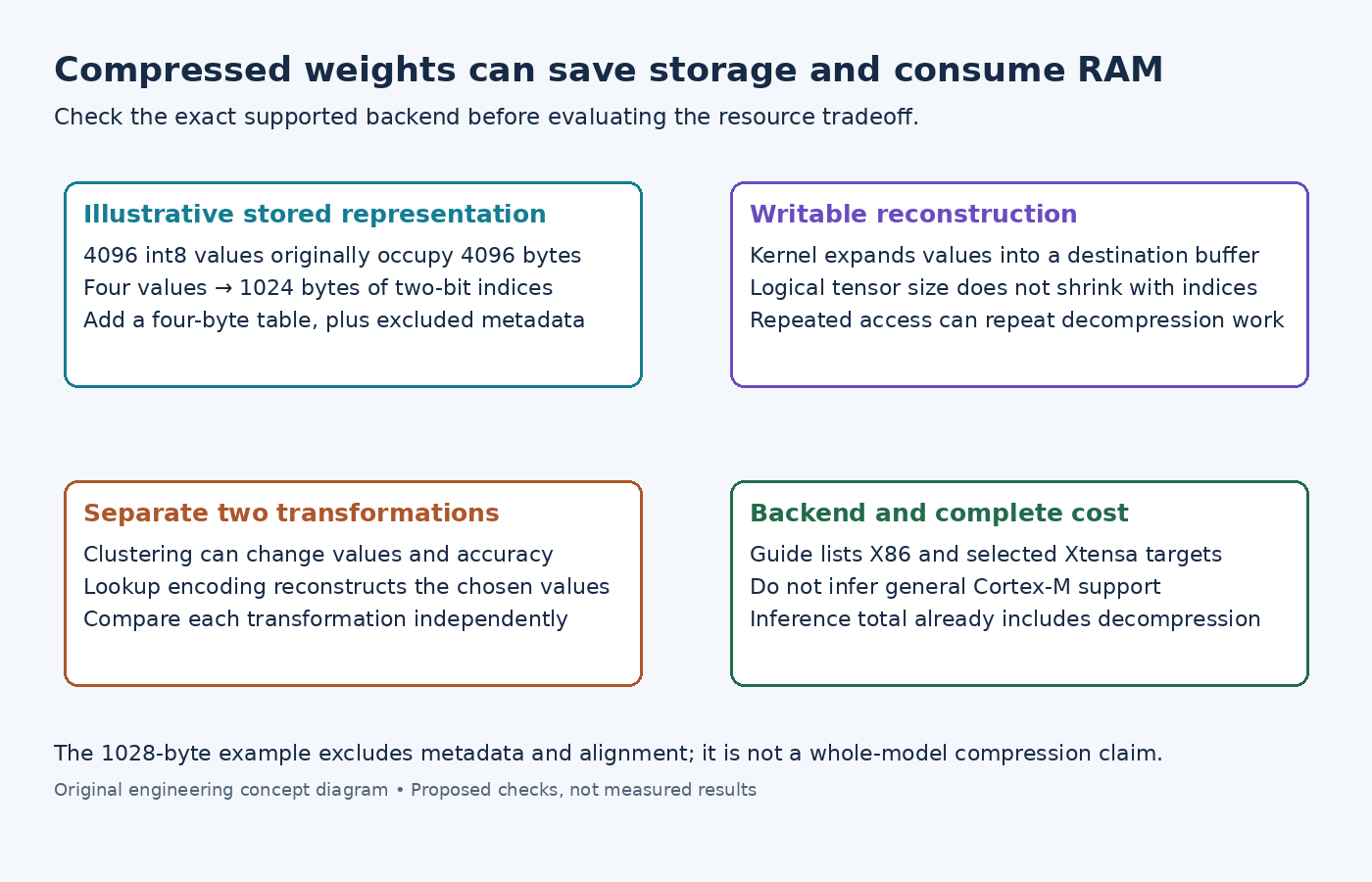
For an illustrative per-tensor int8 array with 4096 elements and four distinct values, two-bit indices occupy 1024 bytes and the four int8 table entries occupy another four bytes. The original values occupied 4096 bytes. This comparison excludes FlatBuffer metadata, alignment and any other tensors; it is not the size reduction of an entire model.

Per-channel tables add their own storage and padding. A tensor with many distinct values can yield much less benefit than a clustered tensor. Inspect the complete exported artifact rather than applying an ideal fourfold factor to total firmware size.

Distinguish value clustering from lossless encoding

Packing indices into a table of the existing values can reconstruct those values exactly. A preceding clustering or binning step changes values to make fewer distinct entries and can change model behavior. The guide explicitly separates that accuracy tradeoff from the encoding mechanism.

Compare the original model with the clustered, uncompressed model to assess value changes. Then compare that model with its compressed representation on the supported execution path. Combining both transformations in one comparison makes it harder to identify whether a discrepancy comes from changed weights or decompression integration.

Inspect where the writable memory is requested

The examined transpose-convolution kernel requests decompression scratch for compressed filter and bias tensors during preparation, under USE_TFLM_COMPRESSION. During evaluation it accesses those tensors through compression-aware helpers.

The helper implementation obtains the decompression destination and reconstructs data on access. The compressed payload's small byte count therefore does not bound the writable capacity needed for its full logical tensor. Repeated helper calls can also repeat decompression work; do not assume a permanent decoded-weight cache.

Alternate decompression regions are an explicit option. The interpreter interface requires configuring them before tensor allocation and keeping the region-description array alive for the interpreter. Their storage still counts toward the product's RAM budget.

Compare the complete tradeoff on the intended target

The generic benchmark guide reports arena use and decompression timing. Its decompression time is already included in ordinary inference timing, so adding the two totals would double-count that work.

Use a supported target to compare final storage, peak writable requirements and complete inference time with identical inputs. Keep correctness and accuracy checks alongside those resource results. No model was compressed or benchmarked here; the decision is whether saved storage is worth the measured memory and execution cost for the particular backend.